ED formulas (2)

Symbol Convention

Symbol Convention%

In accordance with ISO 80000-2, the following font conventions are employed:
- Scalars and components for vectors or tensors are represented by lightface italic type ( $a, ϕ, a_{i}, T_{i j}$ ).
- Vectors are represented by boldface italic type ( $a, ω$ ).
- Second-order tensors are represented by boldface sans-serif type ( $T, I$ ).
- Operators & Constants: Roman (upright) type is used for fixed mathematical constants (e.g., Pi $π$ , the imaginary unit $i$ ) and differential operators (e.g., the differential $d$ in $d x$ ).
- Calculus Notation: For integrals, a thin space (\,) is used to separate the integrand from the differential operator, e.g., $\int f (x) d x$ .
Minkowski Metric: The Minkowski metric tensor $η_{μ ν}$ is defined using the mostly-plus signature convention:

η_{μ ν} = diag (- 1, + 1, + 1, + 1)

Consequently, the invariant spacetime interval is given by $d s^{2} = - c^{2} d t^{2} + d x^{2} + d y^{2} + d z^{2} = - d τ^{2}$ .

Lorentz transformation

K^{'} \to K : x^{α} = Λ_{β}^{α} x^{' β}

For $x$ -axis boost (where $K^{'}$ moves with velocity $v {\hat{e}}_{x}$ relative to $K$ ), the transformation matrix $Λ$ is:

Λ_{β}^{α} = [\begin{matrix} γ & γ β \\ γ β & γ \\ 1 \\ 1 \end{matrix}]

1 Electrostatic Field

1.1 Multipole expansion

Consider electrostatic potential expansion at an external observation point $x$ , with localized charge source $ρ (x^{'})$ confined within a volume $V^{'}$ , and $R = x - x^{'}, r = | x | (f i e l d), r^{'} = | x^{'} | (s o u r c e)$ , then

\begin{aligned} \frac{1}{R} = \frac{1}{| x - x^{'} |} = e^{- x^{'} \cdot \nabla} \frac{1}{r} & = [1 - x^{'} \cdot \nabla + \frac{1}{2!} (x^{'} x^{'} : \nabla \nabla) + \dots] \frac{1}{r} \\ I : \nabla \nabla \frac{1}{r} = 0 ⟹ & = \frac{1}{r} - x^{'} \cdot \nabla \frac{1}{r} + \frac{1}{6} (3 x^{'} x^{'} - r^{' 2} I) : \nabla \nabla \frac{1}{r} + \dots \end{aligned}

⇓

\begin{aligned} φ (x) = \frac{1}{4 π ϵ_{0}} \int \frac{d q}{R} & = \frac{1}{4 π ϵ_{0}} [Q - p \cdot \nabla + \frac{1}{6} D : \nabla \nabla + \dots] \frac{1}{r} \\ = \frac{Q}{4 π ϵ_{0} r} + \frac{p \cdot \hat{r}}{4 π ϵ_{0} r^{2}} + \frac{D : \hat{r} \hat{r}}{8 π ϵ_{0} r^{3}} + \dots \end{aligned}

Where $Q = \int d q = \int ρ (x^{'}) d V^{'}$ is total charge, $p = \int x^{'} d q$ is electric dipole moment, $D = \int (3 x^{'} x^{'} - r^{' 2} I) d q$ is electric quadrupole moment.

Electrostatic intensity expansion

E = - \nabla φ = \frac{Q \hat{r}}{4 π ϵ_{0} r^{2}} + \frac{3 (p \cdot \hat{r}) \hat{r} - p}{4 π ϵ_{0} r^{3}} + \frac{5 (D : \hat{r} \hat{r}) \hat{r} - 2 D \cdot \hat{r}}{8 π ϵ_{0} r^{4}} + \dots

1.2 Small charged body in electric field

Assuming the charge of charged bodies $x$ is so small compared with the source $x^{'}$ which generates the electric field that $\nabla^{2} φ (x) = 0$ . Let $ξ$ be the relative coordinate of a charge element $d q$ from the body's center $x$ . The potential energy $U = \int φ (x + ξ) d q$ of the small body is,

U \approx Q φ |_{x} + p \cdot \nabla φ |_{x} + \frac{1}{6} D : \nabla \nabla φ |_{x} = (Q φ) |_{x} - (p \cdot E) |_{x} - \frac{1}{6} (D : \nabla E) |_{x}

Note that $Q = \int d q = \int ρ (ξ) d V$ , $p = \int ξ d q$ , $D = \int (3 ξ ξ - ξ^{2} I) d q$ are intrinsic properties of the small charged body itself, not the external source.

Furthermore, The total electrostatic force $F$ acting on the small charged body is,

F = - \nabla U = Q E_{ext} |_{x} + (p \cdot \nabla) E_{ext} |_{x} + \frac{1}{6} (D : \nabla \nabla) E_{ext} |_{x} + \dots

The total force moment $N$ acting on the small charged body about its center $x$ is,

N = \int ξ \times E_{ext} (x + ξ) d q = p \times E_{ext} + \frac{1}{3} \nabla \cdot (D \times E_{ext}) + \dots

1.3 Spherical harmonic expansion

1.3.1 Orthonormal Complete Set of Functions

Definition

Orthonormality

\int_{a}^{b} ψ_{n}^{*} (x) ψ_{m} (x) d x = δ_{n m}, with Integration Limits [a, b]

Completeness: Any square-integrable function $f (x)$ can be expanded as

f (x) = \sum_{n} C_{n} ψ_{n} (x), where C_{n} = \int_{a}^{b} ψ_{n}^{*} (x) f (x) d x

which implies

\sum_{n} ψ_{n}^{*} (x^{'}) ψ_{n} (x) = δ (x - x^{'})

Trigonometric & Complex Exponential Functions

ψ_{n} (x) = \frac{1}{\sqrt{a}} \sin \frac{n π x}{a}, \frac{1}{\sqrt{a}} \cos \frac{n π x}{a}, \frac{1}{\sqrt{2 a}} \exp (i \frac{n π x}{a}), with Integration Limits [- a, a]

Note: $n \in N_{+}$ for sine set; $n \in N$ for cosine set; $n \in Z$ for complex set.

Legendre Polynomials

ψ_{l} (x) = \sqrt{\frac{2 l + 1}{2}} P_{l} (x), l \in N, with Integration Limits [- 1, 1]

P_{l} (x) = \frac{1}{2^{l} l!} \frac{d^{l}}{d x^{l}} (x^{2} - 1)^{l} = {\begin{cases} 1, l = 0 \\ x, l = 1 \\ \frac{1}{2} (3 x^{2} - 1), l = 2 \\ \frac{1}{2} (5 x^{3} - 3 x), l = 3 \\ \dots \end{cases}

Spherical Harmonics

ψ_{l m} (θ, φ) = Y_{l}^{m} (Ω) = \sqrt{\frac{1}{2 π} \frac{2 l + 1}{2} \frac{(l - m)!}{(l + m)!}} P_{l}^{m} (\cos θ) e^{i m φ},

l \in N, m \in Z & | m | \leq l, with θ \in [0, π], φ \in [0, 2 π]

P_{l}^{m} (x) = (- 1)^{m} (1 - x^{2})^{\frac{m}{2}} \frac{d^{m}}{d x^{m}} P_{l} (x), for m \geq 0

For negative $m$ , the relations are given by:

P_{l}^{- m} (x) = (- 1)^{m} \frac{(l - m)!}{(l + m)!} P_{l}^{m} (x) or Y_{l}^{- m} (θ, φ) = (- 1)^{m} Y_{l}^{m *} (θ, φ)

The first few associated Legendre functions are,

\begin{aligned} P_{0}^{0} (x) & = 1, \\ P_{1}^{0} (x) & = x, P_{1}^{1} (x) = - \sqrt{1 - x^{2}}, \\ P_{2}^{0} (x) & = \frac{1}{2} (3 x^{2} - 1), P_{2}^{1} (x) = - 3 x \sqrt{1 - x^{2}}, P_{2}^{2} (x) = 3 (1 - x^{2}), \\ P_{3}^{0} (x) & = \frac{1}{2} (5 x^{3} - 3 x), P_{3}^{1} (x) = - \frac{3}{2} (5 x^{2} - 1) \sqrt{1 - x^{2}}, P_{3}^{2} (x) = 15 x (1 - x^{2}), P_{3}^{3} (x) = - 15 (1 - x^{2})^{3 / 2} \\ \dots \end{aligned}

And the first few spherical harmonics are,

\begin{aligned} Y_{0}^{0} (θ, φ) & = \sqrt{\frac{1}{4 π}}, \\ Y_{1}^{0} (θ, φ) & = \sqrt{\frac{3}{4 π}} \cos θ, Y_{1}^{1} (θ, φ) = - \sqrt{\frac{3}{8 π}} \sin θ e^{i φ}, \\ Y_{2}^{0} (θ, φ) & = \sqrt{\frac{5}{16 π}} (3 \cos^{2} θ - 1), Y_{2}^{1} (θ, φ) = - \sqrt{\frac{15}{8 π}} \sin θ \cos θ e^{i φ}, Y_{2}^{2} (θ, φ) = \sqrt{\frac{15}{32 π}} \sin^{2} θ e^{2 i φ}, \\ Y_{3}^{0} (θ, φ) & = \sqrt{\frac{7}{16 π}} (5 \cos^{3} θ - 3 \cos θ), Y_{3}^{1} (θ, φ) = - \sqrt{\frac{21}{64 π}} (5 \cos^{2} θ - 1) \sin θ e^{i φ}, \\ Y_{3}^{2} (θ, φ) & = \sqrt{\frac{105}{32 π}} \cos θ \sin^{2} θ e^{2 i φ}, Y_{3}^{3} (θ, φ) = - \sqrt{\frac{35}{64 π}} \sin^{3} θ e^{3 i φ} \\ \dots \end{aligned}

Orthonormality

\oint Y_{l^{'}}^{m^{'} *} (Ω) Y_{l}^{m} (Ω) d Ω = δ_{l l^{'}} δ_{m m^{'}}

Completeness

\sum_{l = 0}^{+ \infty} \sum_{m = - l}^{l} Y_{l}^{m} (Ω^{'}) Y_{l}^{m} (Ω) = δ (Ω - Ω^{'}) = δ (\cos θ - \cos θ^{'}) δ (φ - φ^{'})

1.3.2 Multipole expansion (Legendre function) *

By using the Legendre generating function, one finds

\frac{1}{R} = \frac{1}{| x - x^{'} |} = \sum_{l = 0}^{\infty} \frac{r_{<}^{l}}{r_{>}^{l + 1}} P_{l} (\cos γ), γ = \arccos \frac{x \cdot x^{'}}{| x \cdot x^{'} |}, r_{<} = min (x, x^{'}), r_{>} = max (x, x^{'})

P_{l} (\cos γ) = 2 π \cdot \frac{2}{2 l + 1} \cdot \sum_{m = - l}^{l} Y_{l}^{m *} (θ^{'}, φ^{'}) Y_{l}^{m} (θ, φ)

Consider a localized charge distribution $ρ (x^{'})$ confined within a volume $V^{'}$ . The exact electrostatic potential $Φ (x)$ at an external observation point $x$ (where $r = | x | > r^{'} = | x^{'} |$ , hence $r_{<} = r^{'}$ and $r_{>} = r$ ) is given by,

Φ (x) = \frac{1}{4 π ε_{0}} \int_{V^{'}} \frac{ρ (x^{'})}{| x - x^{'} |} d^{3} x^{'} = \frac{1}{4 π ε_{0}} \sum_{l = 0}^{\infty} \frac{1}{r^{l + 1}} \int_{V^{'}} ρ (x^{'}) (r^{'})^{l} P_{l} (\cos γ) d^{3} x^{'}

Monopole Term (Point Charge). For $l = 0$ , since $P_{0} (\cos γ) = 1$ , the first term simplifies to:

Φ^{(0)} (x) = \frac{1}{4 π ε_{0} r} \int_{V^{'}} ρ (x^{'}) d^{3} x^{'} = \frac{1}{4 π ε_{0}} \frac{q}{r}, with q = \int_{V^{'}} ρ (x^{'}) d^{3} x^{'}

Dipole Term. For $l = 1$ , since $P_{1} (\cos γ) = \cos γ = \frac{x \cdot x^{'}}{r r^{'}}$ , the second term becomes:

Φ^{(1)} (x) = \frac{1}{4 π ε_{0} r^{2}} \int_{V^{'}} ρ (x^{'}) r^{'} (\frac{x \cdot x^{'}}{r r^{'}}) d^{3} x^{'} = \frac{1}{4 π ε_{0}} \frac{p \cdot \hat{r}}{r^{2}}

with p = \int_{V^{'}} ρ (x^{'}) x^{'} d^{3} x^{'}

Quadrupole Term. For $l = 2$ , since $P_{2} (\cos γ) = \frac{1}{2} (3 \cos^{2} γ - 1)$ , substituting $\cos γ$ into the expression yields:

\begin{aligned} Φ^{(2)} (x) & = \frac{1}{4 π ε_{0} r^{3}} \int_{V^{'}} ρ (x^{'}) (r^{'})^{2} \cdot \frac{1}{2} [3 \frac{(x \cdot x^{'})^{2}}{r^{2} (r^{'})^{2}} - 1] d^{3} x^{'} \\ = \frac{1}{8 π ε_{0} r^{5}} x_{i} x_{j} \int_{V^{'}} ρ (x^{'}) [3 x_{i}^{'} x_{j}^{'} - δ_{i j} (r^{'})^{2}] d^{3} x^{'} \\ = \frac{1}{4 π ε_{0}} \frac{1}{2 r^{5}} \sum_{i, j} D_{i j} x_{i} x_{j} \\ = \frac{D : \hat{r} \hat{r}}{8 π ϵ_{0} r^{3}} \end{aligned}

with D_{i j} = \int_{V^{'}} ρ (x^{'}) [3 x_{i}^{'} x_{j}^{'} - δ_{i j} (r^{'})^{2}] d^{3} x^{'}

And extending to $l = 3, 4, \dots$ yields the octupole ( $l = 3$ ), hexadecapole ( $l = 4$ ), and more high $2^{l}$ -pole moments $\dots$

1.3.3 Rotation of harmonics & Wigner $D$ -Matrices *

See Appendix for ED formulas#2 Rotation of harmonics & Wigner $D$ -Matrices *.

1.4 Method: separation of variables

For this section, everyone is advised to review more example problems.

1.4.1 Cartesian coordinate system

The fundamental solution of Laplace's equation $\nabla^{2} φ = 0$

\frac{\nabla^{2} φ}{φ} = \frac{1}{X} \frac{d^{2} X}{d x^{2}} + \frac{1}{Y} \frac{d^{2} Y}{d y^{2}} + \frac{1}{Z} \frac{d^{2} Z}{d z^{2}} = 0

Let:

\frac{1}{X} \frac{d^{2} X}{d x^{2}} = - k_{x}^{2}, \frac{1}{Y} \frac{d^{2} Y}{d y^{2}} = - k_{y}^{2}, \frac{1}{Z} \frac{d^{2} Z}{d z^{2}} = k_{z}^{2}, k_{z}^{2} = k_{x}^{2} + k_{y}^{2}

Note: The sign of the separation constant is entirely determined by the boundary conditions: directions bounded in space require a negative sign to yield trigonometric functions that can zero out at both boundaries, while directions extending to infinity require a positive sign to yield exponential functions (such as the wave propagating in the z-direction).

In directions where the separation constant is negative (e.g., $x, y$ ),

X (x) = A \cos (k_{x} x) + B \sin (k_{x} x)

In the direction where the separation constant is positive (e.g., $z$ ),

Z (z) = C \cosh (k_{z} z) + D \sinh (k_{z} z)

See the thought from ppt int Appendix for ED formulas#3 Example 2D Laplace Equation in a Rectangular Pipe.

1.4.2 Cylindrical coordinate system

The fundamental solution of Laplace's equation $\nabla^{2} φ = 0$

\frac{1}{s R} \frac{d}{d s} (s \frac{d R}{d s}) + \frac{1}{s^{2} Φ} \frac{d^{2} Φ}{d ϕ^{2}} + \frac{1}{Z} \frac{d^{2} Z}{d z^{2}} = 0

$z$ -direction equation: $\frac{1}{Z} \frac{d^{2} Z}{d z^{2}} = k^{2} ⟹ Z (z) = e^{\pm k z}$ (or monotonic hyperbolic functions)
$ϕ$ -direction equation: $\frac{1}{Φ} \frac{d^{2} Φ}{d ϕ^{2}} = - ν^{2} ⟹ Φ (ϕ) = A \cos (ν ϕ) + B \sin (ν ϕ)$

Note: Since $ϕ$ possesses a $2 π$ periodicity in physical space (i.e., $Φ (ϕ) = Φ (ϕ + 2 π)$ ), the separation constant $ν$ must be an integer.

$s$ -direction equation (Bessel Equation): $\frac{d^{2} R}{d s^{2}} + \frac{1}{s} \frac{d R}{d s} + (k^{2} - \frac{ν^{2}}{s^{2}}) R = 0$

The solutions to this equation are the Bessel functions of the first kind $J_{ν} (k s)$ and the Bessel functions of the second kind (Neumann functions) $N_{ν} (k s)$ . If the physical domain includes the origin ( $s = 0$ ), the coefficient of $N_{ν} (k s)$ must be 0 because $N_{ν} (k s) \to - \infty$ as $s \to 0$ .

Axisymmetric & $z$ -Independent Case ( $ν = 0, k = 0$ )

The Laplace equation collapses to a 1D ODE:

\frac{d}{d s} (s \frac{d φ}{d s}) = 0 ⟹ \frac{d^{2} φ}{d s^{2}} + \frac{1}{s} \frac{d φ}{d s} = 0

$z$ -Independent Case (General Solution for $k = 0$ ):

The problem reduces to a 2D Laplace equation in polar coordinates, where the radial equation transitions from a Bessel equation to an Euler-Cauchy equation,

s^{2} \frac{d^{2} R}{d s^{2}} + s \frac{d R}{d s} - ν^{2} R = 0

the general solution for $k = 0$ is obtained by superimposing all possible harmonic components:

φ (s, ϕ) = \underset{as ν = 0}{\underset{⏟}{A_{0} + B_{0} \ln s}} + \sum_{ν = 1}^{\infty} (A_{ν} s^{ν} + B_{ν} s^{- ν}) \cos (ν ϕ) + \sum_{ν = 1}^{\infty} (C_{ν} s^{ν} + D_{ν} s^{- ν}) \sin (ν ϕ)

1.4.3 Spherical coordinate system

In the spherical coordinate system $(r, θ, ϕ)$ , Laplace's equation is given by,

\nabla^{2} φ = \frac{1}{r^{2}} \frac{\partial}{\partial r} (r^{2} \frac{\partial φ}{\partial r}) + \frac{1}{r^{2} \sin θ} \frac{\partial}{\partial θ} (\sin θ \frac{\partial φ}{\partial θ}) + \frac{1}{r^{2} \sin^{2} θ} \frac{\partial^{2} φ}{\partial ϕ^{2}} = 0

Let the solution be $φ (r, θ, ϕ) = R (r) Θ (θ) Φ (ϕ)$ . Usually, the angular parts are combined and expressed in terms of spherical harmonics (See 3-D Laplace Equation And Spherical Harmonic Function).

Radial Equation

\frac{d}{d r} (r^{2} \frac{d R}{d r}) = l (l + 1) R ⟹ R (r) = A r^{l} + B r^{- (l + 1)}

where $l$ is a non-negative integer.

Angular Equation
- Azimuthal angle $ϕ$ direction: Similar to the cylindrical system, the solution is $e^{\pm i m ϕ}$ (where $m$ is an integer, and $| m | \leq l$ ).
- Polar angle $θ$ direction: Corresponds to the associated Legendre equation, whose solutions are the associated Legendre polynomials $P_{l}^{m} (\cos θ)$ .
Axisymmetric Systems ( $\partial / \partial ϕ = 0 ⟹ m = 0$ )

φ (r, θ) = \sum_{l = 0}^{\infty} (A_{l} r^{l} + \frac{B_{l}}{r^{l + 1}}) P_{l} (\cos θ)

General Case Solution

φ (r, θ, ϕ) = \sum_{l = 0}^{\infty} \sum_{m = - l}^{l} (A_{l m} r^{l} + \frac{B_{l m}}{r^{l + 1}}) Y_{l}^{m} (θ, ϕ)

[\frac{1}{\sin θ} \frac{\partial}{\partial θ} (\sin θ \frac{\partial}{\partial θ}) + \frac{1}{\sin^{2} θ} \frac{\partial^{2}}{\partial ϕ^{2}}] Y_{l}^{m} = - l (l + 1) Y_{l}^{m}, \frac{\partial^{2}}{\partial ϕ^{2}} Y_{l}^{m} = - m^{2} Y_{l}^{m}

1.4.4 Green function

Main equation

\nabla^{2} φ (r) = - \frac{ρ (r)}{ϵ_{0}}

\nabla^{2} G (r, r^{'}) = - \frac{δ (r - r^{'})}{ϵ_{0}}

Fundamental solution in infinite space,

G_{0} (r, r^{'}) = \frac{1}{4 π ϵ_{0} | r - r^{'} |}

φ (r) = \int ρ (r^{'}) G (r, r^{'}) d^{3} r^{'}

With boundaries (Dirichlet condition):

When $φ |_{S} = φ_{0} (r)$ , and the Green's function satisfies

\nabla^{2} G (r, r^{'}) = - \frac{δ (r - r^{'})}{ϵ_{0}}, G (r, r^{'}) |_{r \in S} = 0

then the solution for any volume charge density $ρ$ is,

φ (r) = \int_{V} ρ (r^{'}) G (r, r^{'}) d^{3} r^{'} - ϵ_{0} \oint_{S} φ_{0} (r^{'}) \frac{\partial G (r, r^{'})}{\partial n^{'}} d S^{'}

the green function above is so-called 1-st Green function, which satisfies symmetric condition,

G (r, r^{'}) = G (r^{'}, r)

Note: The Green's function defined in the region $V$ can be understood as the electric potential generated jointly by a point charge placed anywhere inside $V$ and the image charges that satisfy the corresponding boundary conditions.

With boundaries (Neumann condition):

When $\frac{\partial φ}{\partial n} |_{S} = g (r)$ , the Neumann Green's function $G_{N}$ satisfies

\nabla^{2} G_{N} (r, r^{'}) = - \frac{δ (r - r^{'})}{ϵ_{0}}, {\frac{\partial G_{N}}{\partial n} |}_{r \in S} = - \frac{1}{ϵ_{0} S}

the potential is,

φ (r) = \int_{V} ρ (r^{'}) G_{N} (r, r^{'}) d^{3} r^{'} + ϵ_{0} \oint_{S} g (r^{'}) G_{N} (r, r^{'}) d S^{'} + ⟨ φ ⟩_{S}

where $⟨ φ ⟩_{S}$ is the average potential on the boundary.

Refer to Green Function for several basic examples in infinite space.
Refer to ppt for several basic examples with boundary.

1.5 Cases

If all charges are contained within the sphere $V$ (see Appendix for ED formulas#1 $ iiint_V boldsymbol{E}( boldsymbol{x}) , mathrm{d} 3x = - frac{ boldsymbol{p}}{3 epsilon_0}$ or T 2.3 in the textbook)

∭_{V} E (x) d^{3} x = - \frac{p}{3 ϵ_{0}}

An ellipsoid uniformly charged with Q (in the principal inertia axis frame)

D_{11} = \frac{Q}{5} (2 a_{1}^{2} - a_{2}^{2} - a_{3}^{2}), D_{22} = \dots, D_{i \neq j} = 0

2 Magnetostatic Field

2.1 Magnetic energy

#todo -

2.2 Multipole expansion (scalar potential)

2.2.1 magnetic scalar potential

Without free/conductive current

\nabla \times H = J_{f} ⟹ \nabla \times H = 0, H = - \nabla ψ

then for linear media $B = μ H$ ,

\nabla \cdot H = 0 ⟹ \nabla^{2} ψ = 0

Consequently, the multipole expansion can be applied to magnetic scalar potential $ψ$ to derive $H$ as well.

For a current-carrying coil,

ψ (x) = - \frac{I}{4 π} Ω, Ω = - \iint_{S} \frac{\hat{R} \cdot d σ^{'}}{R^{2}}

where $S = \frac{1}{2} \oint_{C} x^{'} \times d l^{'}$ is the arbitrary geometric vector area enclosed by the current loop, and $Ω$ is the solid angle of the surface $S$ with respect to field point $x$ .

2.2.2 Multipole expansion

Consider magnetostatic potential expansion at an external observation point $x$ , with localized current coil/source $J (x^{'})$ confined within a volume $V^{'}$ , and $R = x - x^{'}, r = | x | (f i e l d), r^{'} = | x^{'} | (s o u r c e)$ , then

\begin{aligned} \frac{1}{R} = \frac{1}{| x - x^{'} |} = e^{- x^{'} \cdot \nabla} \frac{1}{r} & = [1 - x^{'} \cdot \nabla + \dots] \frac{1}{r} = \frac{1}{r} - x^{'} \cdot \nabla \frac{1}{r} + \dots \end{aligned}

⇓

\begin{aligned} ψ (x) = \frac{I}{4 π} \iint_{S} \frac{\hat{R} \cdot d σ^{'}}{R^{2}} & = - \frac{I}{4 π} \iint_{S} d σ^{'} \cdot \nabla (\frac{1}{R}) \\ = - \frac{I}{4 π} [(\iint_{S} d σ^{'}) \cdot \nabla - (\iint_{S} d σ^{'} x^{'}) : \nabla \nabla + \dots] \frac{1}{r} \\ = \frac{m \cdot \hat{r}}{4 π r^{2}} + \frac{D_{m} : \hat{r} \hat{r}}{8 π r^{3}} + \dots \end{aligned}

Where there is no magnetic monopole term ( $1 / r$ ). $m = \frac{1}{2} \oint x^{'} \times d I = I \iint_{S} d σ^{'}$ is the magnetic dipole moment of the shell (area vector), and $D_{m} = I \iint_{S} [3 (d σ^{'} x^{'} + x^{'} d σ^{'}) - 2 (x^{'} \cdot d σ^{'}) I]$ is the trace-free magnetic quadrupole moment tensor.

Magnetostatic intensity expansion ( $H = - \nabla ψ$ )

H = \frac{3 (m \cdot \hat{r}) \hat{r} - m}{4 π r^{3}} + \frac{5 (D_{m} : \hat{r} \hat{r}) \hat{r} - 2 D_{m} \cdot \hat{r}}{8 π r^{4}} + \dots

2.3 Multipole expansion (vector potential)

The quadrupole moment of the magnetic field is relatively difficult to calculate and can be skipped. However, the dipole moment needs to be understood.

2.3.1 Moment equation for localized current

Using $\nabla \cdot (J r) = (- \partial_{t} ρ) r + J$ ,

∭_{V} J d V = \dot{p}, p = ∭_{V} r d q

Using $\nabla \cdot (J r r) = (- \partial_{t} ρ) r r + J r + r J$ ,

∭_{V} J r = m \times I + \frac{1}{6} \dot{D} + \frac{1}{6} \dot{g} I

where $m = \frac{1}{2} ∭_{V} (r \times J) d V$ is magnetic dipole moment, $D = \int (3 r r - r^{2} I) d q$ is electric quadrupole moment, and $g = ∭ r^{2} d q$ is the trace of the second spatial moment of the charge distribution.

for steady current, using $\partial_{t} ρ = 0$ ,

∭_{V} J d V = 0

∭_{V} J r d V = m \times I ⟹ ∭_{V} J_{i} r_{j} d V = - ϵ_{i j k} m_{k}

2.3.2 Multipole expansion

Consider magnetostatic potential expansion at an external observation point $x$ , with localized current source $J (x^{'})$ confined within a volume $V^{'}$ , and $R = x - x^{'}, r = | x | (f i e l d), r^{'} = | x^{'} | (s o u r c e)$ , then

\begin{aligned} \frac{1}{R} = \frac{1}{| x - x^{'} |} = e^{- x^{'} \cdot \nabla} \frac{1}{r} & = [1 - x^{'} \cdot \nabla + \frac{1}{2!} (x^{'} x^{'} : \nabla \nabla) + \dots] \frac{1}{r} \\ I : \nabla \nabla \frac{1}{r} = 0 ⟹ & = \frac{1}{r} - x^{'} \cdot \nabla \frac{1}{r} + \frac{1}{6} (3 x^{'} x^{'} - r^{' 2} I) : \nabla \nabla \frac{1}{r} + \dots \end{aligned}

⇓

\begin{aligned} A (x) & = \frac{μ_{0}}{4 π} \int_{V^{'}} \frac{J (x^{'})}{R} d V^{'} \\ = \frac{μ_{0}}{4 π} {\frac{1}{r} \int_{V^{'}} J (x^{'}) d V^{'} + \frac{1}{r^{3}} \int_{V^{'}} J (x^{'}) x^{'} d V^{'} \cdot x + \frac{1}{6} \int_{V^{'}} J (x^{'}) [(3 x^{'} x^{'} - r^{' 2} I) : \nabla \nabla \frac{1}{r}] d V^{'} + \dots} \\ using Coulomb Gauge \to & = \frac{μ_{0}}{4 π r^{3}} (m \times I) \cdot x + \frac{μ_{0}}{24 π} \nabla \times \frac{D_{m} \cdot x}{r^{3}} + \dots \\ = \frac{μ_{0}}{4 π r^{2}} (m \times \hat{r}) - \frac{μ_{0}}{8 π r^{3}} \hat{r} \times (D_{m} \cdot \hat{r}) + \dots \end{aligned}

Where $m = \frac{1}{2} \int_{V^{'}} (x^{'} \times J (x^{'})) d V^{'}$ is the magnetic dipole moment, and $D_{m} = \int_{V^{'}} [(x^{'} \times J) x^{'} + x^{'} (x^{'} \times J)] d V^{'}$ is the trace-free magnetic quadrupole moment tensor.

Magnetostatic intensity expansion

B (x) = \nabla \times A = \frac{μ_{0}}{4 π r^{3}} [3 (m \cdot \hat{r}) \hat{r} - m] + \frac{μ_{0}}{8 π r^{4}} [5 (D_{m} : \hat{r} \hat{r}) \hat{r} - 2 D_{m} \cdot \hat{r}] + \dots

2.3.3 Cases

Ring current

m = I S

where $S = \frac{1}{2} \oint_{C} r \times d l$ is the geometric vector area enclosed by the current loop.

Moving point charge, using $J (r) = q v δ (r - r_{e})$ ,

m = \frac{q}{2 m_{p}} L

where $L = m_{p} (r \times v)$ is the orbital angular momentum.

Rotating charged body, using $J = ρ_{e} (ω \times r)$ , and for any rigid body with $\frac{ρ_{e}}{ρ_{m}} \equiv \frac{Q}{M}$ ,

m = \frac{Q}{2 M} L, L = \int ρ_{m} (r \times v) d V = I_{m} ω

where $I_{m}$ is the moment of inertia tensor. For a sphere with constant $ρ_{e} = \frac{Q}{4 π a^{3} / 3}$ , $I_{m} = \frac{2}{5} M a^{2}$ , thus

m = \frac{1}{5} Q a^{2} ω

for a spherical shell with constant $σ_{e} = \frac{Q}{4 π a^{2}}$ , $I_{m} = \frac{2}{3} M a^{2}$ , thus

m = \frac{1}{2} \oint (r \times K) d σ = \frac{1}{3} Q a^{2} ω

If all currents are contained within the sphere $V$ (see Appendix for ED formulas #1 $ iiint_V boldsymbol{E}( boldsymbol{x}) , mathrm{d} 3x = - frac{ boldsymbol{p}}{3 epsilon_0}$)

∭_{V} B (x) d^{3} x = \frac{2 μ_{0}}{3} m

2.4 Small current-carrying conductor in magnetic field

Assuming the spatial size of the current-carrying body $x$ is so small compared with the distance to the source $x^{'}$ which generates the magnetic field that $\nabla \times B_{ext} = 0$ and $\nabla \cdot B_{ext} = 0$ within the body. Let $ξ$ be the relative coordinate of a current element $J (ξ) d V$ from the body's center $x$ . The interaction magnetic energy $U = \int J (ξ) \cdot A (x + ξ) d V$ of the small body is,

U \approx m \cdot B_{ext} |_{x} + \frac{1}{6} D_{m} : \nabla B_{ext} |_{x} + \dots

Note that $m = \frac{1}{2} \int (ξ \times J (ξ)) d V$ and $D_{m}$ are the magnetic dipole and quadrupole moment tensor, which are intrinsic properties of the small current-carrying body itself, not the external source.

Furthermore, for a system with constant currents, the total magnetostatic force $F$ acting on the small current-carrying body is given by the generalized force relation $F = + \nabla U$ (why use "+"? see Appendix for ED formulas#4 Physical Interpretation of the Sign and Energy Definitions *),

F = + \nabla U = (m \cdot \nabla) B_{ext} |_{x} + \frac{1}{6} (D_{m} : \nabla \nabla) B_{ext} |_{x} + \dots

For a current loop/coil $m = I S$ ,

m \cdot \nabla B = I \nabla (B \cdot S) = I \nabla Φ

The total force moment $N$ acting on the small current-carrying body about its center $x$ is,

N = \int ξ \times (J (ξ) \times B_{ext} (x + ξ)) d V = m \times B_{ext} + \dots

3 Electromagnetic Radiation

3.1 retarded potential

Green function for Wave in infinite space

\partial_{β} \partial^{β} A^{α} = - μ_{0} J^{α}, under gauge \partial_{α} = A^{α} = 0

⟹ {\begin{cases} ◻ G ({\bar{x}}^{μ}) = - δ^{4} ({\bar{x}}^{μ}) \\ G ({\bar{x}}^{μ}) |_{| {\bar{x}}^{μ} | \to \infty} = 0 \end{cases}

where $\bar{x^{μ}} = x^{μ} - x^{' μ}$ . For the derivation process, refer to Green Function or ppt.

Retarded potential (using Lorenz gauge)

A^{μ} (x, t) = \frac{μ_{0}}{4 π} \int \frac{J^{μ} (x^{'}, t_{r})}{| x - x^{'} |} d^{3} x^{'}

or,

φ (x, t) = \frac{1}{4 π ϵ_{0}} \int \frac{ρ (x^{'}, t_{r})}{| x - x^{'} |} d^{3} x^{'}, A (x, t) = \frac{μ_{0}}{4 π} \int \frac{J (x^{'}, t_{r})}{| x - x^{'} |} d^{3} x^{'}

where $t_{r} = t - \frac{R}{c}$ is the retarded time, and $R = x - x^{'}$ . These formulas indicate that the potentials at the field point $x^{μ}$ are determined by the source distribution $J^{μ}$ at an earlier time $t_{r}$ , accounting for the time $\frac{R}{c}$ required for the electromagnetic signal to travel from the source to the field point.

Note: retarded potential satisfied Lorenz gauge.

Retarded EMF (Jefimenko formulas)

E (x, t) = - \nabla φ (x, t) - \frac{\partial A (x, t)}{\partial t} = \frac{1}{4 π ϵ_{0}} ∭ (\underset{coulomb}{\underset{⏟}{ρ_{r} \frac{\hat{R}}{R^{2}}}} + \underset{r a d i a t i o n f i e l d}{\underset{⏟}{{\dot{ρ}}_{r} \frac{\hat{R}}{c R} - \frac{\dot{J_{r}}}{R}}}) d V

B (x, t) = \nabla \times A (x, t) = \frac{μ_{0}}{4 π} ∭ (\underset{Biot-Savart}{\underset{⏟}{\frac{J_{r}}{R^{2}}}} + \underset{radiation field}{\underset{⏟}{\frac{\dot{J_{r}}}{c R}}}) \times \hat{R} d V

3.1.1 Radiation power definition

Angular radiation power

\frac{d P}{d Ω} = r^{2} S_{r} = r^{2} \cdot \frac{1}{μ_{0}} (E_{rad} \times B_{rad}) \cdot \hat{r}

Total radiation power

P = \oint_{Ω} \frac{d P}{d Ω} d Ω

Spherical shell integral (useful when calculating $P$ ). For $\hat{r} = n_{i} {\hat{e}}_{i}$ ,

\oint f (n) d Ω = {\begin{aligned} 4 π, & f & = 1 \\ 0, & f & = n_{i} \\ \frac{4 π}{3} δ_{i j}, & f & = n_{i} n_{j} \\ 0, & f & = n_{i} n_{j} n_{k} \\ \frac{4 π}{5} δ_{(i j} δ_{k l)}, & f & = n_{i} n_{j} n_{k} n_{l} (where δ_{(i j} δ_{k l)} = \frac{1}{3} (δ_{i j} δ_{k l} + δ_{i k} δ_{j l} + δ_{i l} δ_{j k})) \\ ⋮ & ⋮ \\ 0, & f & = n_{i_{1}} n_{i_{2}} \dots n_{i_{2 m + 1}} \\ \frac{4 π}{2 m + 1} δ_{(i_{1} i_{2}} δ_{i_{3} i_{4}} \dots δ_{i_{2 m - 1} i_{2 m})}, & f & = n_{i_{1}} n_{i_{2}} \dots n_{i_{2 m}} \end{aligned}

3.1.2 Time-varying dipole

Density

ρ (x^{'}, t) = - p (t) \cdot \nabla δ^{3} (x^{'}), J (x^{'}, t) = \dot{p} (t) δ^{3} (x^{'})

Potential

A (x, t) = \frac{μ_{0}}{4 π} ∭ \frac{\dot{p} (t - R / c) δ^{3} (x^{'})}{| x - x^{'} |} d V^{'} = \frac{μ_{0}}{4 π} \frac{{\dot{p}}_{r}}{r}, p_{r} = p (t - r / c)

φ (x, t) = \frac{1}{4 π ϵ_{0}} ∭ \frac{- p_{r} \cdot \nabla δ^{3} (x^{'})}{| x - x^{'} |} d V^{'} = - \frac{1}{4 π ϵ_{0}} \nabla \cdot \frac{p_{r}}{r} = \frac{1}{4 π ϵ_{0}} (\frac{p_{r} \cdot \hat{r}}{r^{2}} + \frac{{\dot{p}}_{r} \cdot \hat{r}}{c r})

EMF ( $r > 0$ )

{\begin{aligned} E & = \frac{1}{4 π ϵ_{0}} [\frac{3 (p_{r} \cdot \hat{r}) \hat{r} - p_{r}}{r^{3}} + \frac{3 ({\dot{p}}_{r} \cdot \hat{r}) \hat{r} - {\dot{p}}_{r}}{c r^{2}} + \frac{({\ddot{p}}_{r} \cdot \hat{r}) \hat{r} - {\ddot{p}}_{r}}{c^{2} r}] \\ B & = \frac{μ_{0}}{4 π} (\frac{{\dot{p}}_{r}}{r^{2}} + \frac{{\ddot{p}}_{r}}{c r}) \times \hat{r} \end{aligned}

Poynting vector (for directional dipole $p (t) = p (t) \hat{z}$ )

S = \frac{1}{μ_{0}} E \times B ⟹ {\begin{aligned} S_{r} & = \frac{1}{16 π^{2} ϵ_{0}} [\frac{d}{d t} (\frac{p_{r}^{2}}{2 r^{3}} + \frac{p_{r} {\dot{p}}_{r}}{c r^{2}} + \frac{{\dot{p}}_{r}^{2}}{c^{2} r}) + \frac{{\ddot{p}}_{r}^{2}}{c^{3}}] \frac{\sin^{2} θ}{r^{2}} \\ S_{θ} & = - \frac{1}{32 π^{2} ϵ_{0}} \frac{d}{d t} [{(\frac{p_{r}}{r} + \frac{{\dot{p}}_{r}}{c})}^{2}] \frac{\sin 2 θ}{r^{3}} \\ S_{ϕ} & = 0 \end{aligned}

If $p (t) = p_{0} \cos (ω t)$ , after long-time averaging, the result is simple,

⟨ S_{θ} ⟩ = 0, ⟨ S_{r} ⟩ = \frac{p_{0}^{2} ω^{4}}{32 π^{2} ϵ_{0} c^{3}} \frac{\sin^{2} θ}{r^{2}}

⟨ \frac{d P}{d Ω} ⟩ = r^{2} ⟨ S_{r} ⟩ = \frac{p_{0}^{2} ω^{4}}{32 π^{2} ϵ_{0} c^{3}} \sin^{2} θ

Complex form of resonant dipole

p (t) = p_{0} e^{- i ω t}, p_{0} = p_{0 R} + i p_{0 L}

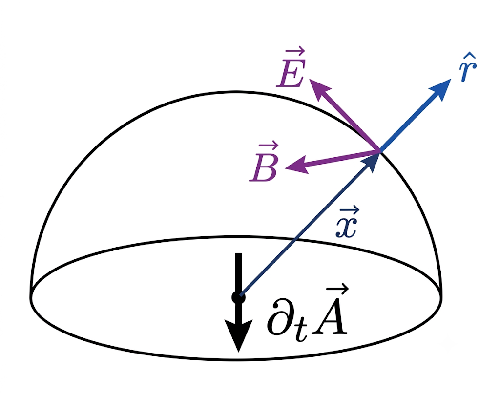
For example, consider a charge pair $\pm e$ separated by distance $2 a$ , rotating anticlockwise around the origin in the $x y$ -plane with constant angular frequency $ω$ so that the positive and negative charges are $r_{\pm} (t) = \pm a \cos (ω t) \hat{x} \pm a \sin (ω t) \hat{y}$ , thus

p (t) = 2 e a (\hat{x} + i \hat{y}) e^{- i ω t}

3.2 Resonant radiation

3.2.1 Far field approximation

For infinitely far field $r^{'} (s o u r c e) ≪ r (f i e l d)$ , one finds

t_{r} = t - \frac{R}{c} \approx t - \frac{r}{c} + \frac{r^{'}}{c} ({\hat{r}}^{'} \cdot \hat{r}) = {\tilde{t}}_{r} + \frac{r^{'}}{c} ({\hat{r}}^{'} \cdot \hat{r}) ≜ t^{*}

\frac{\partial t_{r}}{\partial t} = 1, \nabla t_{r} = - \frac{\hat{r}}{c} + \frac{1}{c} O (\frac{r^{'}}{r})

Note: In order to to maintain consistency with the previous sections and avoid confusion, I consistently use $t_{r} = t - \frac{R}{c} \approx t^{*}$ to denote the real retarded time and ${\tilde{t}}_{r} = t - \frac{r}{c}$ for its leading-order approximation, rather than $t_{r} = t - \frac{R}{c}$ before but $t_{r} = t - \frac{r}{c}$ here in the class.

Consequently, for any field function in the radiation zone of the form $f (x, t) \approx \frac{1}{r} g (t^{*})$ , where the leading-order term is $O (1 / r)$ , its gradient can be expanded as,

\nabla f = \nabla (\frac{1}{r}) g (t^{*}) + \frac{1}{r} g^{'} (t^{*}) \nabla t^{*} = - \frac{\hat{r}}{r^{2}} g (t^{*}) + (\nabla t^{*}) \partial_{t} f

By retaining only the dominant $O (1 / r)$ term, we arrive at the operator equivalence,

\nabla ⟷ - \frac{\hat{r}}{c} \partial_{t}

⟹ c B = (\partial_{t} A) \times \hat{r}, E = c B \times \hat{r}

Ponyting vector can be calculated as,

S = \frac{c}{μ_{0}} B^{2} \hat{r} = ϵ_{0} c E^{2} \hat{r}

3.2.2 Resonant radiation

For resonant radiation

J (x^{'}, t) = J_{0} (x^{'}) e^{- i ω t}

⟹ J (x^{'}, t^{*}) = J_{0} (x^{'}) e^{i (k r - ω t) - i k \cdot x^{'}} = J (x^{'}, t) e^{i (k r - k \cdot x^{'})} = J (x^{'}, {\tilde{t}}_{r}) e^{- i k \cdot x^{'}}, \frac{k}{ω} = \frac{\hat{r}}{c}

\nabla ⟷ i k ⟷ - \frac{\hat{r}}{c} \partial_{t}, \partial_{t} ⟷ - i ω

Vector potential and EMF (by retaining only the dominant $O (1 / r)$ term),

A (x, t) = \frac{μ_{0} e^{i k r}}{4 π r} ∭ J (x^{'}, t) e^{- i k \cdot x^{'}} d^{3} x^{'}

⟨ S ⟩ = \frac{1}{2 μ_{0}} ℜ (E^{*} \times B) = \frac{c}{2 μ_{0}} B^{2} \hat{r} = \frac{ϵ_{0} c}{2} E^{2} \hat{r}

where $E$ and $B$ denote the field amplitudes with the factor $e^{i (k r - ω t)}$ omitted.

Aerial radiation

For a thin antenna of length $l$ , the current distribution forms a standing wave given by,

I (t, z) = I_{0} \sin (m π - k | z |) e^{- i ω t}, z \in [- \frac{l}{2}, \frac{l}{2}], m ≜ \frac{l}{2 π / k} = \frac{l}{λ}

Vector potential and EMF (by retaining only the dominant $O (1 / r)$ term),

A (x, t) = \frac{μ_{0} e^{i k r}}{4 π r} \int_{- l / 2}^{l / 2} \hat{z} I (t, z^{'}) e^{- i k z^{'} \cos θ} d z^{'} = \frac{μ_{0} I_{0} e^{i (k r - ω t)}}{2 π k r} \frac{g (θ)}{\sin θ} \hat{z}, g (θ) = \frac{\cos (m π \cos θ) - \cos (m π)}{\sin θ}

E = - i \frac{μ_{0} c I_{0}}{2 π} \frac{e^{i (k r - ω t)}}{r} g (θ) \hat{θ}, c B = E \hat{ϕ}, linear polarization

⟨ S ⟩ = \frac{ϵ_{0} c}{2} E^{2} \hat{r} = \frac{μ_{0} c I_{0}^{2}}{8 π^{2}} \frac{g^{2} (θ)}{r^{2}} \hat{r}

Definition: resistance of antenna ( $R_{rad}$ )

⟨ P ⟩ = \frac{1}{2} I_{max}^{2} R_{rad}

for short antenna discussed above with $m ≪ 1$ ,

R_{rad} \approx 20 π^{2} m^{2}

3.2.3 Small source approximation

Approximation Regime: localized, long-wavelength source in the radiation zone $r^{'} (s o u r c e) ≪ λ ≪ r (f i e l d)$ with $λ = \frac{2 π}{k}$ is the wavelength of the radiation. This implies that $k \cdot x^{'} \sim \frac{x^{'}}{λ} ≪ 1$ and we can taylor-expand $e^{- i k \cdot x^{'}}$ to obtain,

\begin{aligned} A (x, t) & = \frac{μ_{0} e^{i k r}}{4 π r} ∭ J (x^{'}, t) e^{- i k \cdot x^{'}} d^{3} x^{'} \\ = \frac{μ_{0} e^{i k r}}{4 π r} [\dot{p} (t) + \frac{1}{c} \dot{m} (t) \times \hat{r} + \frac{1}{6 c} \hat{r} \cdot \ddot{D} (t) + \dots] \\ = \frac{μ_{0}}{4 π r} [\partial_{t} p ({\tilde{t}}_{r}) + \frac{1}{c} \partial_{t} m ({\tilde{t}}_{r}) \times \hat{r} + \frac{1}{6 c} \hat{r} \cdot \partial_{t}^{2} D ({\tilde{t}}_{r}) + \dots] \end{aligned}

p = \int x^{'} d q, m = \frac{1}{2} \oint x^{'} \times d I, D = \int (3 x^{'} x^{'} - r^{' 2} I) d q

Electric dipole radiation

Potential and EMF

A (x, t) = \frac{μ_{0} e^{i k r}}{4 π r} \dot{p} (t) ⟹ {\begin{aligned} c B & = \frac{μ_{0} e^{i k r}}{4 π r} \ddot{p} (t) \times \hat{r} \\ E & = c B \times \hat{r} \end{aligned}

Radiation

⟨ S ⟩ = \frac{c}{2 μ_{0}} B^{2} \hat{r} = \frac{μ_{0}}{32 π^{2} c} \frac{| \ddot{p} \times \hat{r} |^{2}}{r^{2}}, ⟨ P ⟩ = \oint | ⟨ S ⟩ | r^{2} d Ω = \frac{μ_{0}}{12 π c} | \ddot{p} |^{2}

where $| \ddot{p} \times \hat{r} |$ and $| \ddot{p} |$ denote the amplitudes with the factor $e^{- i ω t}$ omitted.

For example, a directional dipole $p (t) = p_{0} e^{- i ω t} \hat{z}$

c B = - \frac{μ_{0} ω^{2} p_{0}}{4 π r} \sin θ e^{i (k r - ω t)} \hat{ϕ}, E = c B \hat{θ}

⟨ S ⟩ = \frac{μ_{0} p_{0}^{2} ω^{4}}{32 π^{2} c} \frac{\sin^{2} θ}{r^{2}} \hat{r}, ⟨ P ⟩ = \frac{μ_{0}}{12 π c} p_{0}^{2} ω^{4}

Another example, if $p (t) = p_{0} ({\hat{e}}_{x} + i {\hat{e}}_{y}) e^{i ω t}, p_{0} = e a$ (electron in uniform circular motion),

c B = \frac{μ_{0} ω^{2} p_{0}}{4 π r} (- i \hat{θ} + \cos θ \hat{ϕ}) e^{i (k r - ω t)}, E = \frac{μ_{0} ω^{2} p_{0}}{4 π r} (\cos θ \hat{θ} + i \hat{ϕ}) e^{i (k r - ω t)}

⟨ S ⟩ = \frac{μ_{0} p_{0}^{2} ω^{4}}{32 π^{2} c} \frac{1 + \cos^{2} θ}{r^{2}} \hat{r}, ⟨ P ⟩ = \frac{μ_{0}}{12 π c} | e a ({\hat{e}}_{x} + i {\hat{e}}_{y}) |^{2} ω^{4} = \frac{μ_{0} p_{0}^{2} ω^{4}}{6 π c}

Magnetic dipole radiation

Potential and EMF

A (x, t) = \frac{μ_{0} e^{i k r}}{4 π c r} \dot{m} (t) \times \hat{r} ⟹ {\begin{aligned} E & = - \frac{μ_{0} e^{i k r}}{4 π c r} \ddot{m} (t) \times \hat{r} \\ c B & = \hat{r} \times E \end{aligned}

Radiation

⟨ S ⟩ = \frac{c}{2 μ_{0}} B^{2} \hat{r} = \frac{μ_{0}}{32 π^{2} c^{3}} \frac{| \ddot{m} \times \hat{r} |^{2}}{r^{2}} \hat{r}, ⟨ P ⟩ = \frac{μ_{0}}{12 π c^{3}} | \ddot{m} |^{2}

where $| \ddot{m} \times \hat{r} |$ and $| \ddot{m} |$ denote the amplitudes with the factor $e^{- i ω t}$ omitted.

For example, a directional dipole $m (t) = m_{0} e^{- i ω t} \hat{z}$

E = \frac{μ_{0} ω^{2} m_{0}}{4 π c r} \sin θ e^{i (k r - ω t)} \hat{ϕ}, c B = E \hat{θ}

⟨ S ⟩ = \frac{μ_{0} m_{0}^{2} ω^{4}}{32 π^{2} c^{3}} \frac{\sin^{2} θ}{r^{2}} \hat{r}, ⟨ P ⟩ = \frac{μ_{0}}{12 π c^{3}} m_{0}^{2} ω^{4}

Electric quadruple radiation *

Potential and EMF

A (x, t) = \frac{μ_{0} e^{i k r}}{24 π c r} \hat{r} \cdot \ddot{D} (t) ⟹ {\begin{aligned} c B & = \frac{μ_{0} e^{i k r}}{24 π c r} \hat{r} \cdot \overset{⃛}{D} \times \hat{r} \\ E & = c B \times \hat{r} \end{aligned}

Radiation

⟨ S ⟩ = \frac{c}{2 μ_{0}} B^{2} \hat{r} = \frac{μ_{0}}{1152 π^{2} c^{3}} \frac{| \hat{r} \cdot \overset{⃛}{D} \times \hat{r} |^{2}}{r^{2}} \hat{r}, ⟨ P ⟩ = \frac{μ_{0}}{1440 π c^{3}} | \overset{⃛}{D} |^{2}

where $| \hat{r} \cdot \overset{⃛}{D} \times \hat{r} |$ and $| \overset{⃛}{D} |$ denote the amplitudes with the factor $e^{- i ω t}$ omitted.

For example, a planar quadrupole in the $x y$ -plane with $D (t) = D_{0} e^{- i ω t}$ , where the only non-zero components are $D_{x x} = - D_{y y} = Q_{0}$ ,

c B = - \frac{i μ_{0} ω^{3} Q_{0}}{24 π c r} \sin θ [\sin (2 ϕ) \hat{θ} + \cos θ \cos (2 ϕ) \hat{ϕ}] e^{i (k r - ω t)}, E = - \frac{i μ_{0} ω^{3} Q_{0}}{24 π c r} \sin θ [\cos θ \cos (2 ϕ) \hat{θ} - \sin (2 ϕ) \hat{ϕ}] e^{i (k r - ω t)}

⟨ S ⟩ = \frac{μ_{0} Q_{0}^{2} ω^{6}}{1152 π^{2} c^{3}} \frac{\sin^{2} θ [1 - \sin^{2} θ \cos^{2} (2 ϕ)]}{r^{2}} \hat{r}, ⟨ P ⟩ = \frac{μ_{0}}{720 π c^{3}} Q_{0}^{2} ω^{6}

3.3 Moving point charge

Intensity

J^{α} (x^{μ}) = e c \int u^{α} (τ) δ^{4} (x^{μ} - x_{e}^{μ} (τ)) d τ = (ρ c, J)

ρ (x, t) = e δ^{3} (x - x_{e} (t)), J (x, t) = e v (t) δ^{3} (x - x_{e} (t))

3.3.1 Liénard-Wiechert formulas

Liénard-Wiechert potential

φ (x, t) = \frac{1}{4 π ϵ_{0}} \int \frac{ρ (x^{'}, t_{r})}{| x - x^{'} |} d^{3} x^{'} = \frac{e}{4 π ϵ_{0}} {\frac{1}{R (1 - \hat{R} \cdot β)} |}_{t_{r}}, where t_{r} = t - \frac{| x - x_{e} (t_{r}) |}{c}

A (x, t) = \frac{μ_{0}}{4 π} \int \frac{J (x^{'}, t_{r})}{| x - x^{'} |} d^{3} x^{'} = \frac{β (t_{r})}{c} φ (x, t)

proof ? see Appendix for ED formulas#5 Liénard-Wiechert potential

Liénard-Wiechert EMF

\begin{aligned} E (x, t) & = \frac{e}{4 π ϵ_{0} (1 - \hat{R} \cdot β)^{3}} {[\frac{\hat{R} - β}{γ^{2} R^{2}} + \frac{\hat{R} \times ((\hat{R} - β) \times \dot{β})}{c R}]}_{t_{r}} \\ c B (x, t) & = \hat{R} \times E (x, t) \end{aligned}

where $R = | x - x_{e} (t_{r}) |$ . The first term scales as $O (1 / R^{2})$ (velocity field $E_{v}$ ), while the second term scales as $O (1 / R)$ (acceleration/radiation field $E_{r a d}$ ).

3.3.2 EMF of uniformly moving point charge

\begin{aligned} E (x, t) & = \frac{e}{4 π ϵ_{0}} \frac{1 - β^{2}}{(1 - β^{2} \sin^{2} θ)^{3 / 2}} \frac{\hat{R} (t)}{R^{2}} \\ c B (x, t) & = β \times E \end{aligned}

where $θ = ⟨ R (t), β ⟩$ is the angle between present position and the velocity, the former satisfies,

R (t_{r}) - R (t) = β c (t - t_{r}), R (t_{r}) = c (t - t_{r}) ⟹ R (t) = R (t_{r}) - R (t_{r}) β

However, this form is seldom used in practical radiation problems as the total radiated power of the field is zero.

3.3.3 Radiation of moving point charge

Radiation field $E_{r a d}, B_{r a d}, \hat{R} (t_{r})$ form a right-handed orthogonal triad, thus

S (x, t) = \frac{1}{μ_{0}} E_{r a d} \times B_{r a d} = ϵ_{0} c E_{r a d}^{2} \hat{R} (t_{r})

\frac{d P}{d Ω} = \frac{d W_{r a d}}{d t_{r} d Ω} = \frac{d W_{r a d}}{d t d Ω} \frac{\partial t}{\partial t_{r}} = S R^{2} (t_{r}) (1 - \hat{R} (t_{r}) \cdot β)

Non-Relativistic Limit $β ≪ 1$

For the non-relativistic limit ( $β ≪ 1$ ), $1 - \hat{R} (t_{r}) \cdot β \approx 1$ and $| \hat{R} \times ((\hat{R} - β) \times \dot{β}) | \approx \frac{1}{c} | \hat{R} \times a | = \frac{a}{c} \sin θ$ , $θ = ⟨ \hat{R} (t_{r}), β ⟩ \approx ⟨ \hat{R} (t), β ⟩$ . This reduces directly to Larmor's formula,

\frac{d P}{d Ω} = \frac{μ_{0} e^{2}}{16 π^{2} c} a^{2} \sin^{2} θ, P = \oint \frac{d P}{d Ω} d Ω = \frac{μ_{0} e^{2}}{6 π c} a^{2}

Note: This result is consistent with the instantaneous electric-dipole radiation formula for a single charge. By identifying the dipole moment as $p = e x_{e}$ (hence $\ddot{p} = e a$ ), the total power $P = \frac{μ_{0}}{6 π c} | \ddot{p} |^{2}$ yields identical results.

Relativistic Case $β \in (0, 1)$

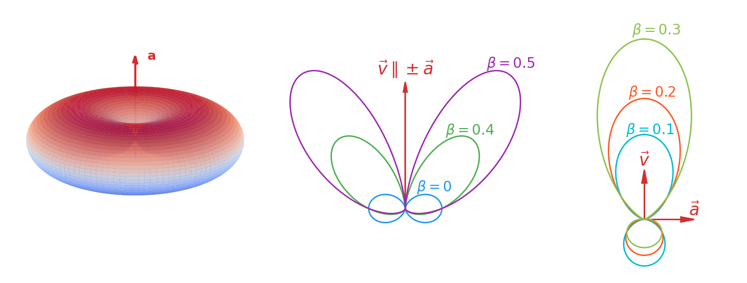
For $β ∥ a$ ( $a = a_{∥} \hat{a}$ ), let $θ = ⟨ \hat{R} (t_{r}), β ⟩$ . The angular radiation distribution becomes,

\frac{d P_{∥}}{d Ω} = \frac{μ_{0} e^{2} a_{∥}^{2}}{16 π^{2} c} \frac{\sin^{2} θ}{(1 - β \cos θ)^{5}}, P_{∥} = \frac{μ_{0} e^{2}}{6 π c} γ^{6} a_{∥}^{2}

As $β \to 1$ (a bit like $θ \to 0$ ), the denominator concentrates the radiation into a sharp forward cone with a characteristic opening angle of $θ_{max} \approx \frac{1}{2 γ}$ .

For $β ⊥ a$ ( $a = a_{⊥} {\hat{e}}_{x}, β = β {\hat{e}}_{z}$ ),

\frac{d P_{⊥}}{d Ω} = \frac{μ_{0} e^{2} a_{⊥}^{2}}{16 π^{2} c} \frac{1}{(1 - β \cos θ)^{3}} [1 - \frac{\sin^{2} θ \cos^{2} ϕ}{γ^{2} (1 - β \cos θ)^{2}}], P_{⊥} = \frac{μ_{0} e^{2}}{6 π c} γ^{4} a_{⊥}^{2}

where $ϕ$ is the azimuthal angle. In the ultrarelativistic limit $β \to 1$ , this expression describes the synchrotron radiation.

The angular radiation distributions for the three conditions discussed above are illustrated below,

The fully relativistic generalization (Liénard's formula), is given by

\frac{d P}{d Ω} = \frac{d P_{∥}}{d Ω} + \frac{d P_{⊥}}{d Ω} + \frac{μ_{0} e^{2} a_{∥} a_{⊥}}{8 π^{2} c} \frac{(β - \cos θ) \sin θ \cos ϕ}{(1 - β \cos θ)^{5}}

P = P_{∥} + P_{⊥} = \frac{μ_{0} e^{2}}{6 π c} γ^{4} [a_{⊥}^{2} + γ^{2} a_{∥}^{2}] = \frac{μ_{0} e^{2}}{6 π c} γ^{6} [a^{2} - {| β \times a |}^{2}]

4-radiation momentum *

Refer to ED Formulas#Primary 4-vector, you could find $P = \frac{μ_{0} e^{2}}{6 π c} a^{μ} a_{μ}$ , which is a Lorentz invariant.

In the particle's instantaneous rest frame, the radiation carries away non-zero energy ( $d E_{rad} = P d τ$ ) but zero 3-momentum ( $d P_{rad} = 0$ ). Thus,

{\frac{d P_{rad}^{α}}{d τ} |}_{r e s t} = (P / c, 0)

Covariantly transfer to the laboratory frame yields,

\frac{d P_{rad}^{α}}{d τ} = (\begin{matrix} γ & γ β \\ γ β & I + (γ - 1) \hat{β} \hat{β} \end{matrix}) (\begin{matrix} P / c \\ 0 \end{matrix}) = \frac{P}{c^{2}} u^{α} = \frac{μ_{0} e^{2}}{6 π c^{3}} (a^{μ} a_{μ}) u^{α}

Lorentz Transformation of $\frac{d P}{d Ω}$ *

Let $K$ be the laboratory frame and $K^{'}$ be the instantaneous rest frame of the moving particle. Let $\frac{d P}{d Ω}$ denote the angular radiation power emitted per retarded time in $K$ , and $\frac{d P^{'}}{d Ω^{'}}$ in $K^{'}$ . The angular distribution transforms as,

\frac{d P}{d Ω} = \frac{1}{γ^{4} (1 - β \cos θ)^{3}} \frac{d P^{'}}{d Ω^{'}} = γ^{2} (1 - β \cos θ^{'})^{3} \frac{d P^{'}}{d Ω^{'}}

where $θ$ (or $θ^{'}$ ) is the angle between the velocity $β$ and the direction of observation in $K$ (or $K^{'}$ ).

proof ? see Appendix for ED formulas#6 Lorentz Transformation of the Angular Distribution of Emitted Radiation Power

Radiation damping *

EM mass of particles

An accelerating charged particle interacts with its own self-field. In the non-relativistic limit, this defines the electromagnetic mass in terms of the electrostatic self-energy $W_{0}$ of the charge distribution,

m_{em} = \frac{4}{3} \frac{W_{0}}{c^{2}}

The rest energy of electron is $W_{0} = \frac{1}{2} \frac{e^{2}}{4 π ϵ_{0} r_{0}}$ for the surface charge shell model, and $W_{0} = \frac{3}{5} \frac{e^{2}}{4 π ϵ_{0} r_{0}}$ for the uniformly charged sphere model. Hence, the observed physical mass $m$ becomes,

m = m_{0} + m_{em}

If we assume that the observed mass of electron is entirely electromagnetic (setting $m_{0} = 0$ ), we could define the classical electron radius $r_{0}$ after ignoring model-dependent geometric factors of order unity,

r_{e} \sim \frac{e^{2}}{4 π ϵ_{0} m c^{2}} \approx 2.818 \times 10^{- 15} m namely \frac{e^{2}}{4 π ϵ_{0} r_{0}} \approx m c^{2}

Why not $W_{0} = m c^{2}$ ? see Appendix for ED formulas#7The $4 / 3$ paradox and Poincaré stresses

Radiation damping

To account for the continuous radiation of 4-momentum, a self-force term $F_{rad}^{μ}$ must be incorporated into the particle's relativistic equation of motion. This yields the Abraham-Lorentz equation,

m \frac{d u^{α}}{d τ} = F_{ext}^{α} + F_{rad}^{α}

By demanding the kinematic consistency condition $u_{α} F_{rad}^{α} = 0$ , the covariant radiation reaction force is derived as,

F_{rad}^{α} = \frac{μ_{0} e^{2}}{6 π c} (\frac{d a^{α}}{d τ} - \frac{1}{c^{2}} (a^{μ} a_{μ}) u^{α})

In the instantaneous rest frame of the particle (or, approximately, for non-relativistic particles as seen in the lab frame), where $u^{α} = (c, 0)$ , $a^{α} = (0, a)$ , and $\frac{d a^{α}}{d τ} = (0, \dot{a})$ , the radiation reaction force decomposes into the time and spatial components,

F_{rad}^{0} = - \frac{μ_{0} e^{2}}{6 π c^{2}} | a |^{2}, F_{rad} = \frac{μ_{0} e^{2}}{6 π c} \dot{a} .

The time component $F_{rad}^{0}$ gives the irreversible radiated power $c F_{rad}^{0} = - \frac{μ_{0} e^{2}}{6 π c} | a |^{2}$ , reproducing the Larmor formula. The spatial component is precisely the Schott term, which has no time component in this frame and hence does no work. It encodes a reversible energy exchange with the near-zone induction fields, which can return energy to the particle when the acceleration $a$ changes.

4 Electromagnetic waves

4.1 EM waves in the medium

4.1.1 Wave equation

The constitutive relations for a homogeneous, isotropic, lossless linear medium, are

D = ϵ E, B = μ H

Maxwell equations in the absence of free sources ( $ρ_{f} = 0$ , $J_{f} = 0$ )

\nabla \cdot D = 0, \nabla \cdot B = 0, \nabla \times E = - \frac{\partial B}{\partial t}, \nabla \times H = \frac{\partial D}{\partial t}

The wave equation

(\nabla^{2} - μ ϵ \frac{\partial^{2}}{\partial t^{2}}) {\begin{matrix} E \\ H \end{matrix}} = 0

The phase and group velocity are,

v = \frac{1}{\sqrt{μ ϵ}} = \frac{c}{n}, with n \equiv \frac{c}{v} = \sqrt{\frac{μ ϵ}{μ_{0} ϵ_{0}}} = \sqrt{μ_{r} ϵ_{r}}

We usually consider non‑magnetic media ( $μ_{r} \approx 1$ ). One has $n \approx \sqrt{ϵ_{r}}$ .

Monochromatic plane‑wave solution

\begin{aligned} E (r, t) & = E_{0} e^{i (k \cdot r - ω t)} = E_{0} e^{i k_{μ} x^{μ}} (physical fields are the real part) \\ H (r, t) & = \frac{1}{ω μ} k \times E, k^{2} = μ ϵ ω^{2} \end{aligned}

define the intrinsic impedance $Z = \frac{ω μ}{k} = \sqrt{\frac{μ}{ϵ}}$ , so $H = \frac{\hat{k} \times E}{Z}$ .

The invariant square of the wave vector $k^{μ} = (ω / c, k)$

k^{μ} k_{μ} = \frac{ω^{2}}{c^{2}} (n^{2} - 1)

In vacuum $n = 1$ and $k^{μ} k_{μ} = 0$ , while inside a typical dielectric $n > 1$ , the wave vector is spacelike ( $k^{μ} k_{μ} > 0$ ), corresponding to a subluminal phase speed.

4.1.2 Energy (flow)

Electromagnetic energy and energy flow

\begin{aligned} w & = \frac{1}{2} ϵ | ℜ (E) |^{2} + \frac{1}{2} μ | ℜ (H) |^{2} = ϵ | ℜ (E) |^{2} = μ | ℜ (H) |^{2} \\ S & = ℜ (E) \times ℜ (H) = \sqrt{\frac{ϵ}{μ}} | ℜ (E) |^{2} = w v_{p} \hat{k} \end{aligned}

The energy transport velocity $v ≜ | S | / w$ equals the phase velocity $v_{p} = c / n$ , which means the energy flows with the wave.

Average energy and energy flow

⟨ w ⟩ = \frac{1}{2} ϵ | E_{0} |^{2} = \frac{1}{2} ϵ E_{0}^{*} \cdot E_{0}, ⟨ S ⟩ = \frac{1}{2} \sqrt{\frac{ϵ}{μ}} | E_{0} |^{2} \hat{k} = ⟨ w ⟩ v_{p} \hat{k}

4.2 EM waves on the surface of the medium

Let medium 1 ( $z < 0$ ) and medium 2 ( $z > 0$ ) be homogeneous, isotropic, lossless linear dielectrics with parameters $ϵ_{1}, μ_{1}$ and $ϵ_{2}, μ_{2}$ . The planar interface is the $z = 0$ plane, with unit normal $\hat{n} = \hat{z}$ pointing into medium 2. A monochromatic plane wave of angular frequency $ω$ is incident from medium 1.

4.2.1 Laws of reflection and refraction

Incident, reflected, and transmitted waves

\begin{aligned} E_{i} (r, t) & = E_{0 i} e^{i (k_{i} \cdot r - ω t)} \\ E_{r} (r, t) & = E_{0 r} e^{i (k_{r} \cdot r - ω t)} \\ E_{t} (r, t) & = E_{0 t} e^{i (k_{t} \cdot r - ω t)} \end{aligned}

with $| k_{i} | = | k_{r} | = k_{1} = n_{1} ω / c$ , $| k_{t} | = k_{2} = n_{2} ω / c$ , and $n_{j} = \sqrt{μ_{j} ϵ_{j} / μ_{0} ϵ_{0}}$ . The corresponding magnetic fields are $H_{j} = (ω μ_{j})^{- 1} k_{j} \times E_{j}$ ( $j = i, r, t$ ).

Boundary condition

\hat{n} \times (E_{2} - E_{1}) = 0, \hat{n} \times (H_{2} - H_{1}) = 0

⟹ (E_{i} + E_{r})_{x, y} = (E_{t})_{x, y} and (H_{i} + H_{r})_{x, y} = (H_{t})_{x, y}

Laws of reflection and refraction

Continuity of the tangential fields at $z = 0$ for all $x, t$ requires the phase factors to match,

k_{i x} = k_{r x} = k_{t x}, ω_{i} = ω_{r} = ω_{t} = ω

Assuming the plane of incidence is the $x z$ -plane. Since $k_{i x} = k_{1} \sin θ_{i}$ , $k_{r x} = k_{1} \sin θ_{r}$ , this gives the law of reflection,

θ_{i} = θ_{r}

With $k_{t x} = k_{2} \sin θ_{t}$ one obtains Snell's law,

n_{1} \sin θ_{i} = n_{2} \sin θ_{t}

4.2.2 Fresnel equations *

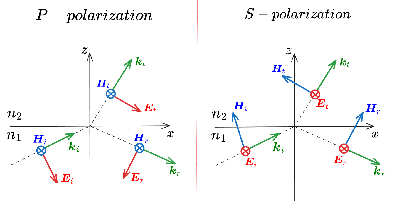
In this section, we follow the reflected convention that reflection reverses the sign of the tangential field parallel to the plane of incidence, while preserving the perpendicular tangential field as the diagram displayed above.

P‑polarization ( $E$ parallel to the plane of incidence)

Let $H_{0 j} = H_{0 j} \hat{y}$ . Tangential $E$ and $H$ (using $H_{0} = (ω μ)^{- 1} k \times E_{0}$ ) continuity gives,

E_{0 i} \cos θ_{i} - E_{0 r} \cos θ_{i} = E_{0 t} \cos θ_{t}, \frac{E_{0 i}}{Z_{1}} + \frac{E_{0 r}}{Z_{1}} = \frac{E_{0 t}}{Z_{2}}

For simplicity, here define the parameters $α ≜ \frac{\cos θ_{t}}{\cos θ_{i}}$ , $β ≜ \frac{k_{2} / μ_{2}}{k_{1} / μ_{1}} = \frac{Z_{1}}{Z_{2}}$ . Solving for $r_{s} ≜ E_{0 r} / E_{0 i}$ and $t_{s} ≜ E_{0 t} / E_{0 i}$ gives,

E_{0 i} - E_{0 r} = α_{w} E_{0 t}, E_{0 i} + E_{0 r} = β E_{0 t}

Solving for $r_{p} ≜ E_{0 r} / E_{0 i}$ and $t_{p} ≜ E_{0 t} / E_{0 i}$ gives,

r_{p} = \frac{β - α}{β + α}, t_{p} = \frac{2}{β + α}

For non‑magnetic media ( $μ_{1} \approx μ_{2} \approx μ_{0}$ ), $β = n_{2} / n_{1}$ , and these reduce to the standard Fresnel formulas.

S‑polarization ( $E$ perpendicular to the plane of incidence)

Let $E_{0 j} = E_{0 j} \hat{y}$ . Tangential continuity gives,

E_{0 i} + E_{0 r} = E_{0 t}, \frac{E_{0 i} - E_{0 r}}{Z_{1}} \cos θ_{i} = \frac{E_{0 t}}{Z_{2}} \cos θ_{t}

which become,

r_{s} = \frac{1 - α β}{1 + α β}, t_{s} = \frac{2}{1 + α β}

Reflectance and transmittance

The power normal to the interface (time‑averaged) defines

R = \frac{⟨ S ⟩_{r, z}}{⟨ S ⟩_{i, z}} = | r |^{2}, T = \frac{⟨ S ⟩_{t, z}}{⟨ S ⟩_{i, z}} = \frac{Z_{1} \cos θ_{t}}{Z_{2} \cos θ_{i}} | t |^{2}

Energy conservation for lossless media ensures $R + T = 1$ . For P or S-polarization,

R_{p} = {(\frac{β - α}{β + α})}^{2}, R_{s} = {(\frac{1 - α β}{1 + α β})}^{2}, T_{p} = T_{s} = \frac{4 α^{2} β^{2}}{(1 + α β)^{2}}

Brewster angle

For P‑polarization, if $θ_{i} + θ_{t} = \frac{π}{2}$ (the same as $r_{p} = 0$ when $α = β$ ) in non‑magnetic media. Together with Snell's law this gives

\tan θ_{B} = \frac{n_{2}}{n_{1}} = β

At this angle the reflected wave is purely S‑polarized.

Assuming $n_{2} > n_{1}$ ( $β > 1$ ). For $θ_{i} < θ_{B}$ ,

α = \frac{\cos θ_{t}}{\cos θ_{i}} = \sqrt{1 + \tan^{2} θ_{i} - {(\frac{\tan θ_{i}}{β})}^{2}} \in (1, β)

⟹ r_{p} > 0, r_{s} < 0

The $s$ component is reversed (phase diff $π$ ) while the $p$ component, referred to the reflected convention, appears unflipped. However, the relative phase between the $p$ and $s$ components changes by $π$ . Hence, the handedness (the sense of rotation from $p$ toward $s$ with thumb along $k$ ) is reversed: an incident left‑handed ellipse becomes right‑handed upon reflection, and vice versa.

For $θ_{i} > θ_{B}$ , $r_{p} < 0, r_{s} < 0$ , both components are $π$ ‑shifted, their relative phase is unchanged, and the handedness remains the same as the incident wave.

Total internal reflection

If $n_{1} > n_{2}$ , Snell's law gives $\sin θ_{t} = (n_{1} / n_{2}) \sin θ_{i}$ . When $θ_{i}$ exceeds the critical angle

θ_{c} = \arcsin (\frac{n_{2}}{n_{1}})

$\sin θ_{t} > 1$ and $\cos θ_{t} = i \sqrt{\sin^{2} θ_{t} - 1}$ becomes purely imaginary. Then $r_{s} = r_{p} = 1$ , the transmitted wave becomes evanescent, and total internal reflection occurs.

More about this phenomenon, see Appendix for ED formulas#8 The evanescent wave.

4.3 EM waves in the conductors

4.3.1 Wave equation

The constitutive relations for a homogeneous, isotropic, linear conductor,

J = σ E, D = ϵ E, B = μ H

Also, inside a homogeneous conductor, any initial free charge accumulation decays exponentially to zero on a timescale of $τ = ϵ / σ$ ( $\sim 10^{- 19} s$ for copper). We can safely assume $ρ_{f} \approx 0$ .

Maxwell equations (assuming $e^{- i ω t}$ time-dependence)

\nabla \cdot E = 0, \nabla \cdot B = 0

\nabla \times E = i ω μ H, \nabla \times H = (σ - i ω ϵ) E = - i ω \tilde{ϵ} E, \tilde{ϵ} = ϵ + i \frac{σ}{ω}

The wave equation

(\nabla^{2} + {\tilde{k}}^{2}) {\begin{matrix} E \\ H \end{matrix}} = 0, {\tilde{k}}^{2} = ω^{2} μ \tilde{ϵ} = ω^{2} μ ϵ + i ω μ σ

To look for plane-wave solutions propagating along the $z$ -direction, we write $\tilde{k}$ in terms of its real and imaginary components,

\tilde{k} = β_{k} + i α_{k}

with β_{k} = ω \sqrt{\frac{μ ϵ}{2}} {[\sqrt{1 + {(\frac{σ}{ω ϵ})}^{2}} + 1]}^{1 / 2}, α_{k} = ω \sqrt{\frac{μ ϵ}{2}} {[\sqrt{1 + {(\frac{σ}{ω ϵ})}^{2}} - 1]}^{1 / 2}, (β_{k}^{2} - α_{k}^{2} = ω^{2} μ ϵ, 2 α_{k} β_{k} = ω μ σ)

The plane wave solution propagating along $\hat{z}$ becomes $E (z, t) = E_{0} e^{- α_{k} z} e^{i (β_{k} z - ω t)}$ .

4.3.2 Good conductor

The good conductor limit

A medium behaves as a good conductor when the conduction current heavily dominates over the displacement current, i.e.,

\frac{σ E}{\partial D / \partial t} \sim \frac{σ}{ω ϵ} = (ω τ)^{- 1} ≫ 1

Under this approximation, the expressions for $β$ and $α$ converge to the same value,

β_{k} \approx α_{k} \approx \sqrt{\frac{ω μ σ}{2}}

The skin depth (The characteristic distance over which the wave's amplitude $E_{0} e^{- α_{k} z}$ attenuates by a factor of $1 / e$ ) is

δ ≜ \frac{1}{α_{k}} \approx \sqrt{\frac{2}{ω μ σ}}

Inside a good conductor, the wave field dies out almost entirely within a few skin depths. For high frequencies, $δ$ is on the order of micrometers, restricting the fields and currents to the very outer edge of the material.

Complex intrinsic impedance

\tilde{Z} = \frac{ω μ}{\tilde{k}} = \frac{ω μ}{β_{k} + i α_{k}}

For a good conductor,

\tilde{Z} \approx \sqrt{\frac{ω μ}{σ}} e^{- i π / 4} = \frac{1}{σ δ} (1 - i)

Hence, for the plane wave solution propagating along $\hat{z}$ : $E (z, t) = E_{0} e^{- α_{k} z} e^{i (β_{k} z - ω t)}$ ,

H (z, t) = \frac{\hat{z} \times E (z, t)}{\tilde{Z}} = E_{0} \sqrt{\frac{σ}{ω μ}} e^{- α_{k} z} e^{i (β_{k} z - ω t + π / 4)} \hat{z} \times E_{0}

Which means: Firstly, $H$ lags behind $E$ by a temporal phase angle of $π / 4$ ; Secondly, The magnetic energy density ( $\frac{1}{2} μ | H |^{2}$ ) is vastly larger than the electric energy density ( $\frac{1}{2} ϵ | E |^{2}$ ) by a factor of $\frac{σ}{ω ϵ}$ , meaning the wave becomes almost purely magnetic.

Good conductors is good reflectors

Consider an electromagnetic wave in a lossless Medium 1 (air with $n_{1} \approx 1$ ) is incident upon a good conductor (Medium 2, with finite but large $σ$ ). The wave vector $k_{t}$ in Medium 2 becomes complex,

{\tilde{k}}_{2} = β_{k} + i α_{k} \approx \frac{1 + i}{δ}

here $δ$ is incredibly small, meaning $| k_{2} | ≫ k_{1}$ . As #P‑polarization ($ boldsymbol{E}$ parallel to the plane of incidence), define the complex parameter $β$ and $α$ ,

\tilde{β} ≜ \frac{k_{2} / μ_{2}}{k_{1} / μ_{1}} \approx \frac{k_{2}}{k_{1}} = \frac{1 + i}{k_{1} δ}, | \tilde{β} | ≫ 1

\sin θ_{t} = (k_{1} / k_{2}) \sin θ_{i} ≪ 1 ⟹ θ_{t} \approx 0 ⟹ α ≜ \frac{\cos θ_{t}}{\cos θ_{i}} \approx \frac{1}{\cos θ_{i}}

For infinite $θ_{i}$ : $| β | ≫ α$ . Therefore,

{\tilde{r}}_{p} = \frac{\tilde{β} - α}{\tilde{β} + α} \to 1, {\tilde{r}}_{s} = \frac{1 - α \tilde{β}}{1 + α \tilde{β}} \to - 1

Which means the good conductor reflects nearly all of the incident field back into Medium 1, and the tangential components of the incident and reflected waves vanish at the interface, also leaving no transmitted wave emerging into the conductor: $\hat{n} \times E_{1} = \hat{n} \times E_{2} = 0$ . Thus, $E$ is normal to the conductor surface, while $H \propto k \times E$ is tangential.

Boundary condition for good conductor ( $\hat{n}$ is pointed to conductor (Medium 2))

\begin{aligned} \hat{n} \times E & = 0 \overset{\nabla \cdot E = 0}{⟹} \frac{\partial E_{n}}{\partial n} = 0 \\ \hat{n} \times H & = - K_{f}, \hat{n} \cdot D = - σ_{f} \\ \hat{n} \cdot H & = 0 \end{aligned}

4.3.3 Resonator

Consider a hollow rectangular cavity with dimensions $0 \leq x \leq a$ , $0 \leq y \leq b$ , and $0 \leq z \leq d$ . The fields inside must satisfy the time-harmonic Helmholtz equation $(\nabla^{2} + k^{2}) E = 0$ , where $k = ω \sqrt{μ ϵ}$ .

Applying the separation of variables under the boundary conditions $\hat{n} \times E = 0, \frac{\partial E_{n}}{\partial n} = 0$ restricts $k$ to discrete values,

k_{x} = \frac{l π}{a}, k_{y} = \frac{m π}{b}, k_{z} = \frac{n π}{d} (l, m, n \in N)

where at most one of the integers can be zero for a given mode. This yields the discrete resonant frequencies of the resonator,

ω_{l m n} = \frac{π}{\sqrt{μ ϵ}} \sqrt{{(\frac{l}{a})}^{2} + {(\frac{m}{b})}^{2} + {(\frac{n}{d})}^{2}}

4.3.4 Waveguide tube

The rectangular waveguide

Consider a hollow waveguide with a rectangular cross-section of width $a$ along the $x$ -axis and height $b$ along the $y$ -axis, with $a > b$ . The inner PEC (perfect electric conductor) walls are located at $x = 0, a$ and $y = 0, b$ . We look for harmonic waves propagating down the tube,

E (r, t) = E_{0} (x, y) e^{i (k_{z} z - ω t)}, H (r, t) = H_{0} (x, y) e^{i (k_{z} z - ω t)}

which satisfy,

(\frac{\partial^{2}}{\partial x^{2}} + \frac{\partial^{2}}{\partial y^{2}} - k_{z}^{2} + k^{2}) {\begin{matrix} E_{0} \\ H_{0} \end{matrix}} = 0

TM Modes (Transverse Magnetic)

For TM waves, the longitudinal magnetic field vanishes ( $H_{z} = 0$ ), and we solve for $E_{0} (x, y)$ . The boundary conditions are,

\begin{aligned} at x = 0, a : E_{z} = E_{y} = \frac{\partial E_{x}}{\partial x} = 0 \\ at y = 0, b : E_{z} = E_{x} = \frac{\partial E_{y}}{\partial y} = 0 \end{aligned}

Applying the separation of variables yields,

\begin{aligned} E_{0 z} (x, y) & = A_{z} \sin (\frac{m π x}{a}) \sin (\frac{n π y}{b}) \\ E_{0 x} (x, y) & = A_{x} \cos (\frac{m π x}{a}) \sin (\frac{n π y}{b}) \\ E_{0 y} (x, y) & = A_{y} \sin (\frac{m π x}{a}) \cos (\frac{n π y}{b}) \end{aligned} (m, n \in N_{0}, and m + n > 0)

Plunging this back into the Helmholtz equation yields the discrete cutoff wavenumber $k_{c}$ ,

k_{c}^{2} = {(\frac{m π}{a})}^{2} + {(\frac{n π}{b})}^{2} = k^{2} - k_{z}^{2}

Crucial Note: If either $m = 0$ or $n = 0$ , the entire field $E_{z}$ collapses to zero. Thus, the lowest-order TM mode is the ${TM}_{11}$ mode.

TE Modes (Transverse Electric)

For TE waves, the longitudinal electric field vanishes ( $E_{z} = 0$ ), and we solve for $H_{0} (x, y)$ . The boundary condition $E_{tangential} = 0$ translates via Maxwell's equations into a Neumann boundary condition for $H_{z}$ (its normal derivative must vanish at the walls),

\begin{aligned} at x = 0, a : E_{y} = H_{x} = 0 ⟹ \frac{\partial H_{z}}{\partial x} = \frac{\partial H_{y}}{\partial x} = 0 \\ at y = 0, b : E_{x} = H_{y} = 0 ⟹ \frac{\partial H_{z}}{\partial y} = \frac{\partial H_{x}}{\partial y} = 0 \end{aligned}

This restricts the solutions to,

\begin{aligned} H_{0 z} (x, y) & = A_{z}^{'} \cos (\frac{m π x}{a}) \cos (\frac{n π y}{b}) \\ H_{0 x} (x, y) & = A_{x}^{'} \sin (\frac{m π x}{a}) \cos (\frac{n π y}{b}) \\ H_{0 y} (x, y) & = A_{y}^{'} \cos (\frac{m π x}{a}) \sin (\frac{n π y}{b}) \end{aligned} (m, n \in N^{+})

The cutoff wavenumber $k_{c}$ shares the exact same algebraic form as the TM modes. However, because cosines do not vanish when their arguments are zero, one of the indices ( $m$ or $n$ ) can safely be zero. Thus, the lowest-order TE mode is the ${TE}_{10}$ or $T E_{01}$ mode.

The Dominant Mode: ${TE}_{10}$

If $a > b$ , the lowest-order TE mode is the ${TE}_{10}$ mode,

k_{c, 10} = \frac{π}{a} ⟹ ω_{c, 10} = \frac{π}{a \sqrt{μ ϵ}} < ω_{c, 01}

The transverse-longitudinal bridge *

This formulation serves as a powerful tool for applying boundary conditions, as well as for deriving all remaining field components once a single longitudinal component is determined.

Using,

\nabla \times E = i ω μ H, \nabla \times H = - i ω ϵ E

Expanding these equations into Cartesian components (replacing $\partial / \partial z$ with $i k_{z}$ ) yields,

\begin{aligned} \frac{\partial E_{z}}{\partial y} - i k_{z} E_{y} & = i ω μ H_{x} \\ i k_{z} E_{x} - \frac{\partial E_{z}}{\partial x} & = i ω μ H_{y} \\ \frac{\partial E_{y}}{\partial x} - \frac{\partial E_{x}}{\partial y} & = i ω μ H_{z} \\ \frac{\partial H_{z}}{\partial y} - i k_{z} H_{y} & = - i ω ϵ E_{x} \\ i k_{z} H_{x} - \frac{\partial H_{z}}{\partial x} & = - i ω ϵ E_{y} \\ \frac{\partial H_{y}}{\partial x} - \frac{\partial H_{x}}{\partial y} & = - i ω ϵ E_{z} \end{aligned}

By solving the simultaneous pairs (1)-(5) and (2)-(4), we form the algebraic bridge that explicitly expresses the transverse field components $(E_{x}, E_{y}, H_{x}, H_{y})$ in terms of the longitudinal components $(E_{z}, H_{z})$ ,

\begin{aligned} E_{x} & = \frac{i}{k_{c}^{2}} (k_{z} \frac{\partial E_{z}}{\partial x} + ω μ \frac{\partial H_{z}}{\partial y}) \\ E_{y} & = \frac{i}{k_{c}^{2}} (k_{z} \frac{\partial E_{z}}{\partial y} - ω μ \frac{\partial H_{z}}{\partial x}) \\ H_{x} & = \frac{i}{k_{c}^{2}} (k_{z} \frac{\partial H_{z}}{\partial x} - ω ϵ \frac{\partial E_{z}}{\partial y}) \\ H_{y} & = \frac{i}{k_{c}^{2}} (k_{z} \frac{\partial H_{z}}{\partial y} + ω ϵ \frac{\partial E_{z}}{\partial x}) \end{aligned}

The general waveguide *

Now we take a hollow tube of any arbitrary cross-section shape into account.

To do this efficiently without solving all 6 components of $E$ and $H$ simultaneously, we split the del operator and the fields into transverse ( $t$ ) and longitudinal ( $z$ ) components,

\nabla = \nabla_{t} + \hat{z} \frac{\partial}{\partial z} = \nabla_{t} + i k_{z} \hat{z}

E = E_{t} + E_{z} \hat{z}, H = H_{t} + H_{z} \hat{z}

By substituting these split forms back into Maxwell's curl equations ( $\nabla \times E = i ω μ H$ and $\nabla \times H = - i ω ϵ E$ ) and separating the components orthogonal to $\hat{z}$ , one obtains,

\begin{aligned} E_{t} & = \frac{i}{k_{c}^{2}} (k_{z} \nabla_{t} E_{z} - ω μ \hat{z} \times \nabla_{t} H_{z}) \\ H_{t} & = \frac{i}{k_{c}^{2}} (k_{z} \nabla_{t} H_{z} + ω ϵ \hat{z} \times \nabla_{t} E_{z}) \end{aligned}

where $k_{c}^{2} ≜ k^{2} - k_{z}^{2} = μ ϵ ω^{2} - k_{z}^{2}$ .

Thus, once you solve the 2D scalar Helmholtz equation $(\nabla_{t}^{2} + k_{c}^{2}) {\begin{matrix} E_{0 z} \\ H_{0 z} \end{matrix}} = 0$ for a given boundary, taking spatial derivatives ( $\nabla_{t}$ ) instantly yields the entire transverse field structure.

The Impossibility of TEM Modes in Hollow Tubes

A TEM (Transverse Electromagnetic) wave requires both $E_{z} = 0$ and $H_{z} = 0$ . Looking at the general decomposition formulas above, if $E_{z} = H_{z} = 0$ , then $E_{t}$ and $H_{t}$ would instantly become zero unless $k_{c}^{2} = 0$ .

If $k_{c}^{2} = 0$ , the transverse electric field reduces to a static-like potential problem: $\nabla_{t}^{2} Φ = 0$ with $E_{t} = - \nabla_{t} Φ$ . For a hollow, single-conductor tube, the entire bounding perimeter forms a single, continuous equipotential surface. By the uniqueness theorem of electrostatics, $Φ = constant$ everywhere inside, meaning $E_{t} = 0$ .

Thus, TEM waves cannot exist inside a hollow, single-conductor waveguide.

Dispersion characteristics

For any chosen mode with a cutoff wavenumber $k_{c}$ , the longitudinal propagation constant is,

k_{z} = \sqrt{k^{2} - k_{c}^{2}} = \sqrt{μ ϵ} \sqrt{ω^{2} - ω_{c}^{2}}, ω_{c} = \frac{k_{c}}{\sqrt{μ ϵ}}

If $ω > ω_{c}$ , $k_{z}$ is real. The wave propagates freely, while for $ω < ω_{c}$ , $k_{z} = i α$ becomes purely imaginary. The fields decay exponentially as $e^{- α z}$ .

Because the wave bounces off the walls rather than traveling in a straight line, the phase fronts and the energy transport move along the axis at different speeds:

Phase Velocity

v_{p} ≜ \frac{ω}{k_{z}} = \frac{c_{m}}{\sqrt{1 - (ω_{c} / ω)^{2}}} > c_{m}, c_{m} = \frac{1}{\sqrt{μ ϵ}}

Group Velocity

v_{g} ≜ \frac{d ω}{d k_{z}} = c_{m} \sqrt{1 - {(\frac{ω_{c}}{ω})}^{2}} < c_{m}

and

v_{p} \cdot v_{g} = c_{m}^{2}

4.4 Lorentz model *

The Lorentz model treats a bound electron in a dielectric as a damped harmonic oscillator driven by the local electric field. We use the same time convention as above, $e^{- i ω t}$ .

4.4.1 Equation of motion for a bound electron

Let $x$ be the displacement of an electron relative to the positive nucleus. For a monochromatic field $E (t) = E_{0} e^{- i ω t}$ ,

m \frac{d^{2} x}{d t^{2}} + m γ \frac{d x}{d t} + m ω_{0}^{2} x = - e E (t)

where $ω_{0}$ is the natural frequency of the bound electron and $γ$ is the damping rate. Therefore,

x_{0} = - \frac{e / m}{ω_{0}^{2} - ω^{2} - i γ ω} E_{0}

The induced dipole moment of one atom is,

p_{0} = - e x_{0} = \frac{e^{2} / m}{ω_{0}^{2} - ω^{2} - i γ ω} E_{0} ≜ α (ω) E_{0}

Thus the atomic polarizability is,

α (ω) = \frac{e^{2} / m}{ω_{0}^{2} - ω^{2} - i γ ω}

4.4.2 Electric susceptibility and dielectric function

If the number density of oscillators is $N$ , then

P = N p = ϵ_{0} χ_{e} (ω) E

so that

χ_{e} (ω) = \frac{N e^{2}}{ϵ_{0} m} \frac{1}{ω_{0}^{2} - ω^{2} - i γ ω} = \frac{ω_{p}^{2}}{ω_{0}^{2} - ω^{2} - i γ ω}, ω_{p}^{2} ≜ \frac{N e^{2}}{ϵ_{0} m}

For several resonance modes,

χ_{e} (ω) = \frac{N e^{2}}{ϵ_{0} m} \sum_{j} \frac{f_{j}}{ω_{0 j}^{2} - ω^{2} - i γ_{j} ω}, \sum_{j} f_{j} \approx 1

where $f_{j}$ is the oscillator strength. The complex permittivity is,

\tilde{ϵ} (ω) = ϵ_{0} [1 + χ_{e} (ω)]

and for a non-magnetic dielectric,

{\tilde{n}}^{2} (ω) = 1 + χ_{e} (ω)

Writing $χ_{e} = χ^{'} + i χ^{″}$ for a single resonance gives,

χ^{'} = ω_{p}^{2} \frac{ω_{0}^{2} - ω^{2}}{(ω_{0}^{2} - ω^{2})^{2} + γ^{2} ω^{2}}, χ^{″} = ω_{p}^{2} \frac{γ ω}{(ω_{0}^{2} - ω^{2})^{2} + γ^{2} ω^{2}}

The real part $χ^{'}$ determines dispersion, while the imaginary part $χ^{″} > 0$ determines absorption.

4.4.3 Dispersion and absorption

Absorption

For weak absorption, write $\tilde{n} = n + i κ$ . A plane wave propagating in the $+ z$ direction is then,

E (z, t) = E_{0} e^{i (\tilde{n} ω z / c - ω t)} = E_{0} e^{- κ ω z / c} e^{i (n ω z / c - ω t)}

so the intensity obeys,

I (z) = I_{0} e^{- a_{a b s} z}, a_{a b s} = \frac{2 κ ω}{c}

The time-averaged absorbed power density is,

⟨ p_{a b s} ⟩ = \frac{ω}{2} ϵ_{0} χ^{″} | E_{0} |^{2} = \frac{ω}{2} Im (\tilde{ϵ}) | E_{0} |^{2}

Near $ω \approx ω_{0}$ , $χ^{″}$ has a peak and the wave is strongly absorbed. Away from resonance, $χ^{″}$ becomes small and the medium is approximately transparent, but $χ^{'}$ still varies with frequency, producing dispersion.

(Anomalous) dispersion

For a weakly absorbing dielectric, $κ ≪ n$ , or equivalently $χ^{″} ≪ χ^{'}$ . From ${\tilde{n}}^{2} = (n + i κ)^{2} = 1 + χ^{'} + i χ^{″}$ one obtains,

n^{2} - κ^{2} = 1 + χ^{'}, 2 n κ = χ^{″}

Therefore, in the weak-absorption limit $κ ≪ n$ ,

n (ω) \approx \sqrt{1 + χ^{'} (ω)}, κ (ω) \approx \frac{χ^{″} (ω)}{2 n (ω)}

Only for a dilute or weakly polarizable medium, $| χ_{e} | ≪ 1$ , can one further expand

n \approx 1 + \frac{1}{2} χ^{'}, κ \approx \frac{1}{2} χ^{″}

The frequency dependence of $n (ω)$ is called dispersion. The phase velocity and group velocity are,

v_{p} = \frac{ω}{k} = \frac{c}{n (ω)}, v_{g} = \frac{d ω}{d k} = \frac{c}{n + ω \frac{d n}{d ω}}

For the Lorentz oscillator,

χ^{'} (ω) = ω_{p}^{2} \frac{ω_{0}^{2} - ω^{2}}{(ω_{0}^{2} - ω^{2})^{2} + γ^{2} ω^{2}}

Hence, below resonance ( $ω < ω_{0}$ ), usually $χ^{'} > 0$ and $n > 1$ ; above resonance ( $ω > ω_{0}$ ), $χ^{'} < 0$ and $n$ decreases. Near resonance, let $δ ≜ ω - ω_{0}$ and assume $| δ | ≪ ω_{0}$ , then

ω_{0}^{2} - ω^{2} \approx - 2 ω_{0} δ

and

χ^{'} (ω) \approx - \frac{2 ω_{p}^{2}}{ω_{0}} \frac{δ}{4 δ^{2} + γ^{2}}, χ^{″} (ω) \approx \frac{ω_{p}^{2} γ}{ω_{0}} \frac{1}{4 δ^{2} + γ^{2}}

Therefore, in the resonant absorption band,

{\frac{d χ^{'}}{d ω} |}_{ω = ω_{0}} \approx - \frac{2 ω_{p}^{2}}{ω_{0} γ^{2}} < 0